Time series forecasting is an important prediction technique that involves projecting future values based on historical data patterns. It is critical in many industries and applications, assisting decision-making and optimising resource allocation.

In this blog, we will look at the notion of time series forecasting, how it differs from time series analysis, and how it is used in practice.

What is Time Series Forecasting?

Forecasting time series is an important field of machine learning (ML) and can be thought of as a supervised learning task. Time series forecasting can be accomplished using a variety of ML methods, including Regression, Neural Networks, Support Vector Machines, Random Forests, and XGBoost. The fundamental goal is to use models that have been fit on past data to predict future observations.

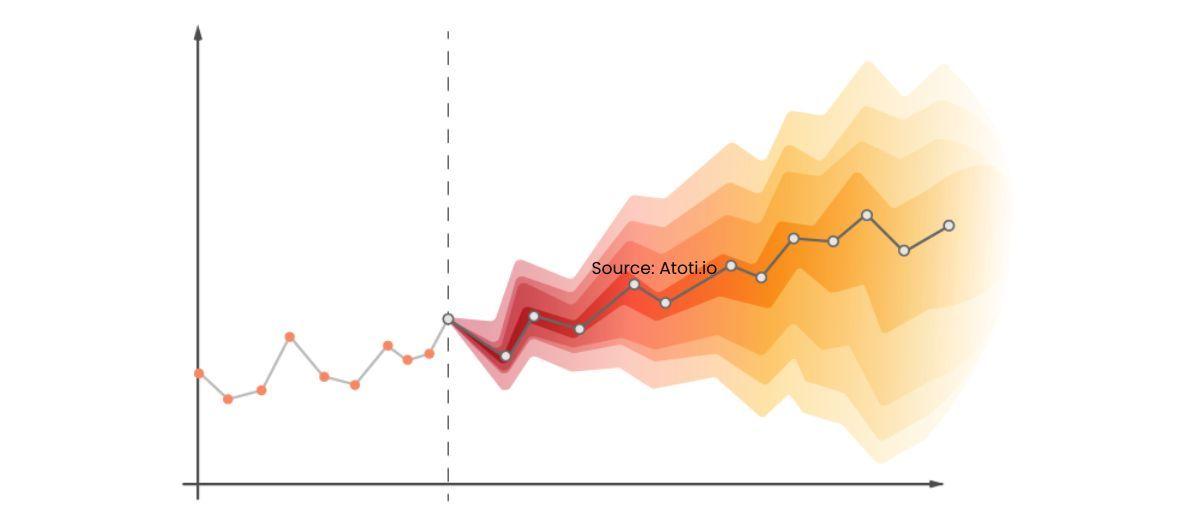
The essence of time series forecasting is projecting future values over a certain time period. It entails creating models based on historical data and using them to create observations that will ultimately influence future strategic decisions.

The future is projected or forecasted in this procedure based on what has previously transpired. Time series data introduces time order dependence between observations, which serves as a constraint as well as a structure that provides crucial additional information.

Time Series Analysis vs. Time Series Forecasting

While time series analysis and time series forecasting are closely related, there is a distinct difference between the two. Time series analysis focuses on understanding the underlying patterns, trends, and statistical properties of the data. It involves techniques such as autocorrelation, trend analysis, and decomposition to gain insights into the data's behavior.

On the other hand, time series forecasting takes the analysis a step further by using historical data to make predictions about future values. Various forecasting methods, such as exponential smoothing, moving averages, and autoregressive integrated moving average (ARIMA) models are commonly employed to estimate future values and identify potential trends or anomalies.

Components of Time Series Analysis

Before embarking on the journey of Time Series Analysis, it's crucial to understand its key components:

1. Trend

Imagine a path without rigid steps, where data points steadily rise, fall, or remain constant. This is the trend – a continuous direction in the dataset. Trends can be positive (upward), negative (downward), or even nonexistent (neutral).

2. Seasonality

Think of the dataset as a repeating pattern over fixed intervals – much like the changing seasons. This is seasonality, where data exhibits regular cycles. These cycles might resemble the graceful curve of a bell or the sharp angles of a sawtooth.

3. Cyclical

Here, there's a more unpredictable rhythm to the data, with no fixed intervals. Imagine waves with varying heights and periods – this is cyclical behavior. It's not as systematic as seasonality and can be influenced by economic, political, or other external factors.

4. Irregularity

Just like sudden surprises in real life, datasets can encounter unexpected spikes due to unforeseen events or situations. These irregularities are short-lived and might not follow any particular pattern.

In summary, time series analysis involves dissecting these components. Trends guide long-term shifts, seasonality reflects repeating patterns, cyclical behavior adds complexity, and irregularities introduce short-lived surprises.

By understanding these components, we unlock insights into past behaviors and potentially predict future trends. So, whether it's for business, economics, or science, mastering time series analysis can illuminate the hidden stories within data.

Types of Time Series Forecasting Models

Time series forecasting is an important part of data analysis that is used to predict future trends and behaviours based on past patterns and data.

There are several types of time series forecasting models that are appropriate for different sorts of data, and each model has strengths and drawbacks that vary depending on the data used for the analysis.

The following are some of the most common time series forecasting models.

1. Autoregressive (AR) Model

The Autoregressive (AR) model predictions future events based on prior values of the same variable. It presupposes that a variable's future value is linearly related to its prior values.

The number of lagged values utilised for prediction is determined by the AR model's order, represented as 'p'. An AR model, for example, predicts the current value using the value from the previous time step. AR models are beneficial when there is a significant correlation between the past and future values of a variable.

An autoregressive model takes the following general form: [latex]Y_t = c + \phi_p Y_{t-p} + \varepsilon_t[/latex]

2. Moving Average (MA) Model

Another sort of time series forecasting methodology is the Moving Average (MA) model. It, like the AR model, predicts future values by using past values of the variable. Instead of directly using the variable's prior values, the MA model computes the variable's average over a predetermined number of time steps. MA models are excellent for detecting short-term trends and smoothing out random oscillations in data.

A moving average model, rather than using prior predicted values in a regression, uses past forecast errors in a regression-like model. MA(q) is the notation for the moving average model of order q:

Where θ= parameters of the model μ= expectation of Xt ε= white noise error terms

3. Autoregressive Moving Average (ARMA) Model

The Autoregressive Moving Average (ARMA) model combines the AR and MA ideas. To create predictions, it takes advantage of the data's autoregressive nature (using prior values) as well as its moving average nature (using past forecast errors).

The ARMA model is specified by two parameters: 'p' for the autoregressive component order and 'q' for the moving average component order. This approach is frequently successful in capturing both short-term and long-term trends in time series data.

4. Vector Autoregressive (VAR) Model

The Vector Autoregressive (VAR) model extends the notion of the AR model to several variables. It is used to forecast the future values of many connected time series variables. The VAR model evaluates variable interactions and makes predictions based on prior values. It is a sophisticated model for analysing and forecasting complicated systems with numerous time series data.

5. Vector Error Correction (VECM) Model

The Vector Error Correction (VECM) model is an extension of the VAR model that takes cointegration among variables into consideration. The long-term equilibrium relationship between variables that may diverge from each other in the short term is referred to as cointegration.

Because the VECM model captures both short-term dynamics and long-term interactions between variables, it is appropriate for predicting in situations where variables are mutually reliant.

Overview of Time Series Forecasting Methods

Time series forecasting is an important method for projecting future patterns in business, finance, and economics for strategic decision-making.

There are several time-series forecasting methods to choose from, each with its own set of advantages and disadvantages.

In this section, we will go through some of the most frequent ways.

1. Time-Series Decomposition

Time-series decomposition is the process of breaking down a time series into its constituent parts: trend, seasonality, and random variations. Understanding and modelling these components individually allows us to get insights into the data's underlying patterns.

The decomposition of a time series allows us to discern the long-term trend, cyclic patterns, and irregular fluctuations. This strategy allows us to create accurate models that capture the numerous factors influencing the data. We can better comprehend the behaviour of the data and generate more trustworthy forecasts by knowing the decomposition of the time series.

2. Time-Series Regression Models

Time-series regression models investigate the relationship between a series of data points and one or more independent variables. When there is a causal relationship between the time series and external factors, these models are especially beneficial.

We can capture the impact of these elements on the time series and create better forecasts by introducing extra information into the study, such as economic indicators or marketing activities.

Depending on the nature of the data and the forecasting problem, time-series regression models can take several forms, such as linear regression, multiple regression, or logistic regression. These models aid in understanding the impact of independent variables on time series and provide useful information for projecting future trends.

3. Exponential Smoothing

For forecasting time series data, exponential smoothing is a popular technique. It assigns decreasing weights to previous observations, giving more weight to newer data items. Exponential smoothing is especially useful for data sets that lack a clear trend or seasonality.

The idea behind exponential smoothing is to capture underlying trends in data by emphasising recent observations and filtering out random oscillations. This method is popular for short-term forecasting since it is simple and computationally efficient.

There are several varieties of exponential smoothing models, including simple exponential smoothing, Holt's linear trend model, and Holt-Winters' seasonal model, each of which is tailored to unique data features.

3. ARIMA Models

In time series forecasting, ARIMA (AutoRegressive Integrated Moving Average) models are commonly utilised. To capture the underlying trends in the data, these models integrate autoregressive (AR), differencing (I), and moving average (MA) components. ARIMA models work especially well with data sets that have trends and seasonality.

The autoregressive component captures the link between the current observation and a set number of previous observations; the moving average component captures the influence of previous forecast errors; and differencing aids in the removal of trends and the stabilisation of the data.

ARIMA models can capture the complicated behaviour of time series data and produce reliable forecasts by combining these three components.

4. Neural Networks

In time series forecasting, neural networks, notably recurrent neural networks (RNNs), have gained appeal. RNNs can recognise complicated patterns and non-linear correlations in data. These models are especially useful for analysing sequential data and can use historical data to predict future values.

RNNs feature a network topology that allows them to take into account temporal dependencies in data, making them appropriate for time series forecasting. However, neural networks frequently demand a large quantity of data for training and may require more computer resources than other methods.

Nonetheless, they have been shown to be useful in a variety of applications, such as weather forecasting, energy demand prediction, and stock market analysis.

5. TBATS

The TBATS (Trigonometric, Box-Cox Transformation, ARMA errors, Trend, and Seasonality) forecasting approach is designed for time series with numerous seasonalities. To capture distinct patterns in the data, it combines components from exponential smoothing, ARIMA models, and trigonometric functions.

TBATS models are effective at managing data with both short-term and long-term seasonalities, making them useful in a variety of practical applications. TBATS models may handle data with non-normal distributions and autocorrelated errors by adding the Box-Cox transformation and ARMA errors. This strategy is especially effective in businesses like retail, where seasonal trends such as daily, weekly, and yearly seasonality occur.

How to analyze Time Series?

In today's data-driven landscape, unlocking the insights hidden within time-dependent data has become an indispensable skill. Time series analysis, a foundational component of data analytics, enables us to interpret trends, estimate future events, and make sound judgements.

Let's get started with a detailed introduction to efficiently analysing time series data.

Step 1: Data collection and cleaning

The first step in any analysis is to gather relevant data and ensure its accuracy. Cleaning the data involves identifying and rectifying anomalies, missing values, and outliers that could distort your analysis. A sound foundation is crucial, as it forms the basis for all subsequent stages.

Step 2: Visualization with Time as the axis

Visualizations provide a powerful means to comprehend the underlying patterns in time series data. Creating plots where time is on the x-axis and the key feature on the y-axis allows us to identify trends, seasonality, and cyclic behaviors that might exist within the data.

Step 3: Testing Stationarity

A series is stationary when its statistical properties, like mean and variance, remain constant over time. Various tests are available to assess stationarity, aiding in the decision to proceed with further analysis or apply transformations if needed.

Step 4: Understanding the nature

Charts like autocorrelation and partial autocorrelation plots help us understand the relationships between data points at different lags. These tools are invaluable in identifying potential patterns and guiding us towards suitable modeling techniques.

Step 5: Model building

Modeling is where the magic happens. Several model types are at your disposal, including AutoRegressive (AR), Moving Average (MA), AutoRegressive Integrated Moving Average (ARIMA), and their variants. Selecting the right model involves considering the data's characteristics and selecting appropriate parameters to achieve accurate predictions.

Step 6: Extracting insights

The ultimate goal of time series analysis is to extract meaningful insights for decision-making. After building the model, it's crucial to evaluate its performance using techniques like backtesting and cross-validation. This step fine-tunes the model and prepares it for prediction.

The Significance of Time Series Analysis in Predictive Insights

Time Series Analysis (TSA) serves as a fundamental tool for predicting and understanding future trends, particularly in scenarios where time plays a crucial role. This technique holds immense value in various industries, from finance to healthcare, as it enables us to extract meaningful insights from historical data.

At its core, TSA involves delving into historical datasets to identify patterns and trends that unfold over time. By grasping these patterns, we can effectively compare current situations and align them with past occurrences. This process allows us to pinpoint the factors influencing specific variables across different time periods.

The true power of "Time Series" lies in its ability to facilitate a wide array of time-based analyses with actionable outcomes:

1. Forecasting

TSA empowers us to make informed predictions about future values. Whether it's predicting stock prices or the demand for a product, this capability is indispensable for making strategic decisions.

2. Segmentation

Grouping similar items together based on time-related patterns can lead to insightful categorizations. This aids in recognizing trends that might not be apparent through other analysis methods.

3. Classification

Time Series Analysis can also be used for classifying items into predefined categories. This classification can help in identifying trends specific to each category over time.

4. Descriptive Analysis

Sometimes, the goal is simply to understand the nature of a dataset. TSA assists in comprehending the composition and characteristics of data spread across different time points.

5. Intervention Analysis

Understanding the impact of changing variables on outcomes is essential. TSA allows us to assess how altering a specific variable influences the overall outcome, helping in decision-making.

Time Series Forecasting Applications

Time series forecasting has numerous applications in a variety of fields. Here are some noteworthy examples:

1. Finance

• Stock market forecasting: Time series forecasting techniques are widely employed to predict future stock prices based on historical trading data. This information is crucial for investors and traders when making investment decisions.

• Foreign exchange rate forecasting: Forecasting future currency exchange rates is essential for international business and finance. Time series forecasting methods help in predicting fluctuations in exchange rates, which enables companies to manage currency risks effectively.

• Demand forecasting: Time series forecasting is utilized in finance to estimate demand for financial instruments like bonds or options. This information helps financial institutions in their decision-making processes related to investments and portfolio management.

2. Supply Chain Management

• Inventory optimization: Time series forecasting plays a vital role in optimizing inventory levels. By predicting future demand for products, businesses can efficiently manage their inventory to avoid overstocking or shortages. This, in turn, helps reduce costs and improve customer satisfaction.

• Demand forecasting: Forecasting customer demand is crucial for supply chain management. By using time series forecasting techniques, businesses can estimate future demand patterns, plan production and procurement activities accordingly, and optimize their supply chain processes.

3. Energy and Utilities

• Load forecasting: Time series forecasting is used in the energy sector to predict energy consumption patterns. By forecasting load demand, utilities can optimize resource allocation, plan for future capacity requirements, and ensure efficient generation, transmission, and distribution of electricity.

• Renewable energy forecasting: Time series forecasting is essential for optimizing the integration of renewable energy sources into the power grid. By accurately predicting renewable energy production, utilities can balance supply and demand, reduce reliance on traditional energy sources, and improve grid stability.

4. Economics

• GDP forecasting: Time series forecasting techniques are employed in economics to predict future economic growth. By analyzing historical data and economic indicators, economists can make forecasts regarding GDP (Gross Domestic Product) growth, which aids in policymaking and economic planning.

• Inflation forecasting: Time series forecasting is used to estimate future inflation rates. By analyzing past inflation patterns and economic indicators, economists can make predictions about inflation trends. This information is valuable for central banks and policymakers to implement appropriate monetary policies.

Time series forecasting provides vital insights into future trends and patterns in each of these applications. It assists organisations and decision-makers in their respective professions in anticipating changes, mitigating risks, optimising resources, and making more informed strategic decisions.

Conclusion

Time series forecasting is a strong tool that allows organizations to generate accurate forecasts and make informed future decisions. Businesses can acquire important insights and plan ahead by exploiting historical data and employing various strategies and models.

While Time Series Analysis is a powerful technique, it is not without limitations. One problem is dealing with missing numbers, as the method's prediction ability is dependent on complete data.

Furthermore, Time Series Analysis assumes linear relationships between data points, which may exclude more complex nonlinear trends. The technique frequently necessitates data modifications, which can be computationally and resource-intensive.

Finally, its primary strength is in univariate cases, as it struggles to accommodate the complicated interplay of many factors. These limitations highlight the necessity for a nuanced approach in which the method's merits are leveraged alongside an understanding of its limits.

Time series forecasting allows you to predict the future, whether it's sales for the next quarter or weather patterns for crop planning. Embrace this fascinating field, and unlock the potential it holds for unravelling the mysteries of time itself.