This is a follow-up article of the previous blog which covers the general high-level architecture of Artificial Neural Networks and the basic overview. You may consider referring to the previous article to get aligned with the discussion of this article.

The concept of understanding how Artificial Neural Networks(ANN) actually work on solving real-life problems can be scary to understand at first. It’s fascinating to see how it extracts the pattern from the input data and maps it with the correct target labels. This is the ideology behind the working of neural networks. The key idea is to explore the feed-forward propagation in a neural network and for this particular blog, backpropagation is considered out of scope.

What are the Different Layers in NN?

We’re restricting our discussions only to dense neural networks where each neuron is connected to other neurons in a network.

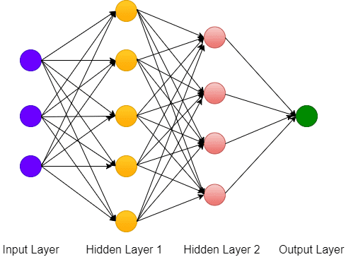
ANN consists of three layers - Input, Hidden and Output. There cannot be more than 1 input and output layer in a network. At Least one hidden layer is a must for ANN architecture.

The fig-1 shows the architecture of a neural network consisting of 3 neurons in the input layer followed by two hidden layers each with 5 and 4 neurons respectively. Finally, we have an output layer with one neuron. Note that output may have more than one neuron in case of multi-classification problems.

The weights and biases are assigned differently at each different layer. We will also explore the role of activation functions used in a layer, in a later section.

What are Weights and Biases in NN?

Weight is perhaps the most important parameter in an ANN. In a loose sense, weights refers to giving some importance to the features.

However, in an ANN, each input is assigned a random weight (normally between 0 and 1). The weight operation is multiplying the input feature by its corresponding random weight.

The bias could be interpreted as the process of triggering a neuron in ANN or to control the triggering of neurons.

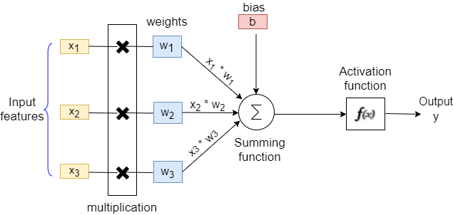
Consider an example of a single neuron as shown below, where there are 3 input features (X1, X2, and 3) with corresponding weights (W1, W2, and W3). We also have a corresponding bias ‘b’ associated with the neuron.

The multiplication of weight with input features followed by the addition of bias is our actual equation representing the first mathematical equation of any neural network structure in general.

The idea of the single neurons can be expanded to a large number of interconnected neurons in an ANN. This model is a prototype of what the large ANN would look like. Here, the output of one neuron serves as an input to neurons in other successive layers, until it reaches the output layer.

What is the Activation Function?

In the above example, we show that the output of a neuron could be possibly expressed as a linear combination of weight ‘w’ and bias ‘b’ as something like w * x + b.

This simple linear combination is not very useful in learning complex patterns from the training data, as it would look like the linear regression model only. The activation function is applied after the summing function in the fig 2.

The Activation function decides if a neuron should be triggered or not for the learning. It squashes the value normally in the region of the proximity of the particular activation function used. y = Activation (Σ(weight * input) + bias)

The popular choice of activation function could be a sigmoid, ReLU or hyperbolic tangent (tanh) functions. In this blog post we’re going to focus only on sigmoid function to understand the basics of all other activation functions in general.

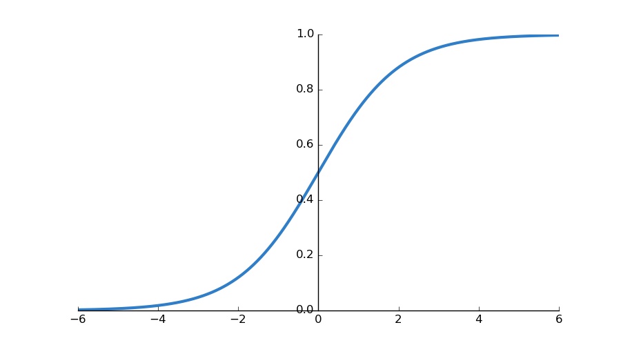
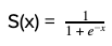
Sigmoid is a S-shaped function as illustrated in the fig 3. The mathematical function of sigmoid is represented by the equation S(x).

By default, the threshold of the function is 0.5 (as shown on the y-axis). It squashes the value between 0 and 1 with respect to the threshold value.

For eg., if the value of S(x) after computing the sigmoid function is less than 0.5, it squashes the value of 0 and if the value of S(x) is equal to or greater than 0.5, it squashes the value to 1.

The sigmoid is preferred mostly at an output layer for binary classification problems. However, if we have multi-classification problems, we can use the SOFTMAX activation function.

The limitation of using sigmoid function is that the neuron's activation saturates at either tail of 0 or 1, the gradient at these regions is almost zero.

The Fundamental Equation of Straight Line

The output of a single neuron can be expressed as a function of a linear combination of ‘w’ and ‘b.’ In another analogy the equation y = w * x + b can be compared with our straight line equation y = mx + c. (‘m’ being the slope of the line and ‘c’ being the intercept of the line).

One can change the values of ‘m’ and ‘c’ to change the steepness and the relative position (with respect to the y-axis) of the line. So, using this concept we could easily solve a simple binary classification problem (0 or 1) by building a decision boundary separating two regions. We would choose the line of best fit (by determining the best possible value of ‘m’ and ‘c’) to differentiate two regions by a simple mathematical line.

Consider an example of solving a binary classification problem using a simple linear classifier as shown in fig 4. We are trying to build a decision boundary separating the two classes indicated by circle and triangle objects.

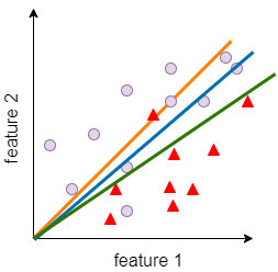
It could be noted that the green color line is a ‘line of best fit’ and it distinguishes two classes in a better way than other lines. However, real life problems are not always so linear in nature and they may even include a large number of features as well. In such a case where the problem involves lots of data, non-linearity and complex features, a Neural Network is the best option to solve the problem.

Forward Propagation Calculation

The process in which information flows forward from one layer to another in a sequential manner is called forward propagation. To understand it more visually, let’s take a look at the following example of what’s really happening at the node of a single neuron. This understanding would give us a clear picture of forward propagation. In our case the activation function f(x) is going to be sigmoid i.e., S(x).

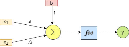
y = g ( Σ (w * x) + b) y = g ((4X1 - 3X2) + 1)

It should be noted that 4X1 - 3X2 + 1 represents the equation of line in 2-dimension! The final step is to apply the sigmoid function to the above equation. For that, let’s assume X1 = 1 and 2 = 3. Our equation turns out to be:

This example can be further extended to all the neurons that are the part of learning in a neural network.

Conclusion

This blog explores the mathematics associated with the feedforward propagation of neural networks. This is just the first step towards gaining intuition on neural networks. It is to be noted that the first feedforward process would generate a predicted output at an output layer. There would always exist some difference between the predicted output and an actual output, referred to as error. In the next article, I will explore how the neural network tries to minimize the error by backpropagation. The feedforward propagation and backpropagation together constitute the training of the model in several iterations until the error is within the accepted thresholds.

References:

1. Neural networks

2. What is neural networks